
A component can pass structural and thermal checks but still fail electromagnetically - wrong torque, uncontained EMI or poor antenna performance.
Unlike FEA or CFD, electromagnetic simulation must account for the space around the product, not just the solid geometry.
CST Studio Suite works with SOLIDWORKS geometry - assign electromagnetic material properties, define sources and mesh the computational domain including the surrounding space.
Electromagnetic losses can feed into thermal analysis, and force density results can transfer to structural simulation.
The engineering process is familiar - define the question, model the system, analyse the response. The adjustment is learning to treat fields and surrounding space as part of the design problem.

Applications Engineer BE in Mechanical Engineering
A component can be strong enough to carry its mechanical loads and still fail to perform as intended. A motor may meet its structural requirements but produce the wrong torque. An electronic enclosure may protect its contents physically but fail to contain electromagnetic interference. These problems cannot be understood from stress, temperature or fluid flow alone.
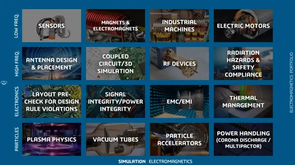
Electromagnetic simulation allows engineers to predict how electric and magnetic fields interact with a product’s geometry and materials. At lower frequencies, that might mean investigating a motor, transformer or electromagnetic actuator. At higher frequencies, the questions shift towards antennas, wave propagation, radiation and electromagnetic interference. For someone accustomed to finite element analysis (FEA) or computational fluid dynamics (CFD), the general process is not new. The engineer starts with a model, assigns materials and operating conditions, creates a mesh and runs a solver. The most important difference is that an electromagnetic field may extend beyond the physical components in the CAD model. Understanding that difference makes the rest of the workflow easier to follow.

An electromagnetic model begins with the geometry of the product. CST Studio Suite can work with SOLIDWORKS geometry, allowing the existing CAD model to form the basis of the electromagnetic study rather than rebuilding the product from scratch.
Reusing the design geometry reduces the need to recreate the product in a separate modelling system. It also helps keep the electromagnetic study aligned with the current design revision. However, the geometry still needs to be prepared for the physical question being investigated, just as it would for an FEA or CFD study.
The engineer must assign the relevant electromagnetic properties to each material. These properties determine how the materials respond to electric and magnetic fields. Sources must also be defined to represent inputs such as current, voltage or an applied field.
Up to this point, the process resembles other forms of simulation. The main difference becomes clear when deciding what the mesh must include.
Consider a transformer containing coils, an iron core and an enclosure. In a structural analysis, the engineer might concentrate on the solid components, their supports and the loads applied to them. An electromagnetic analysis must also account for the magnetic field surrounding those components.
The field can pass through the core, cross gaps and extend into the space around the transformer. That surrounding space therefore forms part of the calculation, even though it is not a manufactured component.
CST represents unassigned space within the model boundary as a background material. The physical components and the background region within the model’s bounding box form the computational domain. The solver calculates the electromagnetic field throughout this domain rather than only inside the solid geometry.
Boundary conditions define how the field behaves at the outer limits of the computational domain. The engineer therefore needs to consider both the physical product and the region through which its fields may travel.
This is the key change in perspective for someone coming from mechanical simulation. The empty space around the CAD model is not necessarily empty from the solver’s point of view. It may be an active part of the electromagnetic problem.
Once the domain, materials, sources, boundaries and mesh have been defined, the next question is what the resulting field calculation can tell the engineer about the design.
The important question isn’t how many result plots CST can produce. It’s whether those results help answer an engineering question. A field plot is useful when it answers a specific design question. Magnetic flux density, for example, shows how the magnetic field is distributed and where it becomes concentrated. In a transformer or electrical machine, this can help the engineer examine whether the field is passing through the expected parts of the design.
Time-varying magnetic fields can induce eddy currents in conducting materials. CST can calculate the distribution of these currents and the losses associated with them. The location of the losses matters because electromagnetic loss can become a source of heat.
Those losses can be transferred to a thermal simulation to calculate the resulting temperature distribution. Electromagnetic force density can also be transferred to a mechanical simulation, while force and torque results can be used when evaluating electrical machines. The electromagnetic study therefore supplies loads that can affect the thermal and structural behaviour of the product.
This relationship is especially useful for mechanical engineers. Electromagnetic simulation does not replace FEA or thermal analysis. It can provide the forces and heat sources that those analyses need when electromagnetic behaviour influences the mechanical design.
At higher frequencies, the engineering questions change. The analysis may focus on how electromagnetic waves propagate, radiate or interfere with an electronic system. For example, an antenna may be structurally perfect and correctly packaged inside an enclosure, but nearby electronics, housing materials or geometry can change how effectively it radiates. Different solvers are used because the underlying behaviour and the required results are different, but the purpose remains the same: determine whether the product’s electromagnetic behaviour supports its intended function.
Simulation can be used during design to investigate that behaviour, compare alternatives and identify areas that may require attention before a prototype is built. Physical testing still has a separate role. It validates the finished design under real operating conditions and checks whether the assumptions made in the simulation were appropriate.
The physics is different, but the engineering logic is consistent: define the question, model the system, analyse the response and use testing to validate the design. For a mechanical engineer moving into electromagnetic simulation, the biggest adjustment isn’t learning a completely different engineering process. It’s learning to think about fields and the space around the product as part of the design problem.
Share this post: